CREx: technical details
the main ingredient of CREx is the common interval tree data structure
(Bérard et al. 07). it is important
to know how to interpret them, in order to get correct results.
common intervals
one way to define similar regions of two gene orders are common intervals
(Uno and Yagiura 2000, Heber
and Stoye 2001). a common interval is a set of genes that appears consecutively
in both given gene orders. Hence, a set of neighbored genes that were not separated during
the evolution of the gene orders is a common interval. (note that the definition says
nothing about the orientation of the genes.) for example consider the gene orders
(A B C D E F G) and (E D G -F A B C). the set {A, B, C} is a common interval because
the genes A, B, and C appear consecutively in both gene orders, while the set {C, D}
is not a common interval (it appears consecutively in gene order 1 but not in gene
order 2). another example of a common interval is {D, E, F, G} - even if gene F
is reversed and the genes are rearranged the genes appear consecutively, so they are a
common interval.
we argue that it could be important to respect the constraints given by common intervals
in the reconstruction of the gene order evolution. one motivation is that the common intervals
represent clusters functionally coupled genes which are preserved during evolution.
another motivation is that if a cluster of genes can be found in two gene orders
- for what reason ever - it likely makes sense to not separate it, i.e. to preserve it. one
further motivation is - as we demonstrate here and elsewhere (e.g.
Bernt at al. 2007) - that the constraints like common intervals have the potential
to simplify the reconstruction of gene order evolution.
In principle, common intervals of gene orders can be computed
efficiently. A problem is that their number can be very large
(in computer science terms O(n²)). this
makes a graphical representation and comparison difficult.
strong common intervals
fortunately there exists a small subset of the common intervals which can be used to
represent the set of all common intervals. these are the so called strong intervals
(Bérard et al. 07).
a strong common interval is a common interval that does not overlap any of the other
common intervals. formally: c ⊂ d, d ⊂ c or c ∩ d = ∅ holds for all
strong common intervals c and d, i.e. two strong intervals are either
disjoint or one is included in the other. the single elements of the gene orders
and the set containing all elements are always strong common intervals.
strong interval tree (pq-tree)
the inclusion order of the strong common intervals can be used to define a tree data structure
(called strong interval tree), where each node represents one strong common
interval. the leaf nodes of this tree are the strong common intervals containing the
single elements and the root node is the strong common interval containing all elements.
there is an edge between two nodes - representing two strong common intervals I and J -
if I ⊂ J and there is no strong common interval K such that I ⊂ K ⊂ J.
based on the order of the children of a node one can define three different node types:
- linear increasing (+) nodes: the children of the nodes appear in the exact same
order in the two gene orders
- linear decreasing (-) nodes: the children of the nodes appear in reversed order
in the two gene order
- prime nodes: all other cases
the leafs of the interval tree - i.e. the single genes - are always linear nodes.
interpretation of strong interval trees / family diagrams
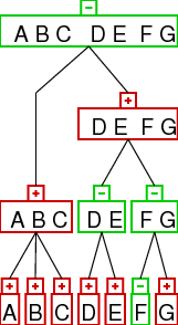
below we present the interval tree (left) and the family diagram (right) for
the above example of two gene orders. the top row shows the diagram/tree relative to
gene order 1 and the bottom row relative to gene order 2.
first the tree:
- each node (box) of the tree represents one of the strong common intervals
- the sign in the little box on top of each node tells the user if the node is
increasing (+) or decreasing, additionally this information is given by the
colors: increasing nodes are red while decreasing nodes are green. (prime nodes
are blue, but there is none such node present in this example)
the family diagram:
- the family diagram is an alternative visualization to the interval
tree. To get an idea just imagine viewing the tree from above (or below).
| interval tree | family diagram |
 |
|
 |
|
|
the interpretation:
- the node type of the leafs (the single genes) represents the sign
of the elements. as you can see it is easy to identify genes of different orientation in
both gene orders: just look for linear decreasing leave nodes (green). in the example
only the F has different orientation
- lets look at the inner node (A B C). it has red color, which means that it is linear increasing. i.e.
the order of its children is the same in both gene orders. as above this can be easily
identified by looking for red inner nodes.
- the inner node (D E) is green, which means it is linear decreasing.
so the order of the children is opposite in the two gene orders. in
gene order 1 the sequence is D E and in gene order 2 the sequence is
E D.
- note that the orientation of the children is unimportant, its all about the relative
order. this is exemplified by node (F G). this node is linear decreasing, which means that
the relative order of the children is different in the two input gene orders. this makes
no statement about the orientation of the children.
- the exact meaning of the words "the order of its children" is very important.
look at node (D E F G), it is an increasing node. this means the in both gene orders
there is first D E followed by F G. the relative order of D and E (resp. F G) is unimportant.
|
rearrangement identification and prime node scenarios
often it is possible to identify rearrangement operations from a given strong
interval tree. we consider inversions (reversals), reverse transpositions,
transpositions, and tdrl rearrangements. the idea is that the rearrangements result in
different patterns in the strong interval tree as demonstrated below.
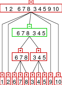
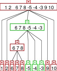
| Inversion | Transposition | Reverse Transposition | TDRL |
 |
 |
 |
 |
the images show the interval trees for a gene order which was generated from the
identity permutation (1,2,3,...) by applying one rearrangement. as you can see the
interval trees produced in this way show different patterns - which can be
detected automatically. the patterns are the following:
- inversion: a linear node with a parent of different orientation and all
children in the same orientation
- transposition: a linear node with exactly two children, the orientation
of the children and the parent has to be opposite to the orientation of the node
- reverse transposition: a linear node with orientation different to the orientation
of the parent. the children have to be of the different orientation followed
by children of the same orientation
- prime nodes: read below
important observation is that tdrl operations always lead to prime nodes. note,
that it is not true to argue that every prime node was generated by a tdrl - another
possibility to generate a prime node is with a rearrangement 'hot spot' (i.e. a region
of the gene order where lots of rearrangements took place). therefore
we have to search for tdrl operations only in prime nodes. the actual tdrl scenario
is computed with the methods presented in Chaudhuri et al. 2006.
unfortunately these methods do not work for signed permutations, i.e. tdrls can not
explain any changes in the orientation of genes. therefore we apply a simple heuristic
search method which incorporates inversions. if a prime node has k contiguous blocks
of decreasing children then we have to apply exactly k inversions to get a prime
node with only increasing children. we try all possibilities to apply these inversions
and select from the resulting permutations those which need a minimal number of
tdrls to sort them. note that the number of those permutations can be very large.
therefore we limit the number of resulting scenarios which we present.
(one additional remark on the tdrl scenarios: transpositions are a trivial kind of tdrls,
if the algorithm that is used to compute the tdrl scenario includes a transposition we mark
this. if there are multiple possible scenarios for a prime node CREx sorts them such
that scenarios which include a larger number of transpositions come first.)
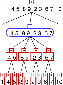
in contrast to inversions, transpositions, and reverse transpositions the
interpretation of a tdrl representation, as given by CREx, is not that easy. therefore
we present an example here.
> one
A B C D E F
> two
B D F A C E
the output of CREx looks like this:
one → two
-
family diagram for one
-
family diagram for two
-
scenario:
|
What does this mean? What is it about the blue and red shaded boxes?
- the first step of a tdrl is a tandem duplication. this step is not shown in the
diagram. in the example: (A B C D E F) is duplicated to: (A B C D E F A B C D E F)
- after the duplication comes the random loss of one copy of each gene. the interesting
information is which copy is lost:
- the elements in the blue shaded boxes are lost in the second copy. therefore the
remaining copies are moved to the front.
- similarly the elements in the red shaded boxes are lost in the first copy.
therefore the remaining copies are moved to the back.
- obviously the tdrl operation creates a prime node (the blue one)
- below the family diagrams of the two permutations you can see the tdrl scenario
|
two → one
-
family diagram for two
-
family diagram for one
-
scenario:
|
an important piece of information is that the tdrl operation is not symmetric.
this is perfectly demonstrated by this example. while we need one tdrl step
for transforming gene order one into gene order two, the other direction needs
two tdrl steps. in this way tdrl rearrangements may provide information about the
direction of the rearrangement. in this case one might conclude that the
direction of the tdrl was from 'one' to 'two'.
|